01 The impulse viewer at a glance

impulse is a powerful visualization and analysis workbench which helps engineers to comfortably understand and debug complex semiconductor and multi-core software systems.

Views

A view combines a freely configurable set of plots organized in the form of a tree.  Users can define multiple views and choose between them at any time to get the information they need.

Plots

Plots are easily configurable specific representations of signal data.  Plots may have a common zoomable and scrollable axis (e.g. the time of the trace) or they may be adjusted into the window size (charts).

Cursors

Cursors allow navigation and measurement within signals.
Users can specify any number of cursors. A dedicated details area shows the current position and delta distances.

To open the viewer, select a wave file of a supported format in the Explorer or Navigator view, and use the context menu to open the file (as you would open a source file for editing). To use the example wave files, select Import->'impulse example wave files' .

H001 Beginners - How to open the viewer

There are multiple ways to view signal data with impulse. You might :

  • Use eclipse file resources :
    1. If no project exists existing, create a new project of any type (File->New->Project->??? );
    2. Import your record files (wave files, logs, traces,..) or drag and drop them into the project;
    3. Double-click the record file to open (or use the context menu of the file).
  • Use the File->Open File ... menu:
    1. Open the menu File->Open File ... ;
    2. Select the file to open;
    3. Press OK.
H002 Beginners - How to import example wave files

impulse come with a set a example wave files.

  1. If no project exists existing, create a new project of any type (File->New->Project->??? );
  2. Open the "Import..." menu (from "File"" menu or from the navigator context menu)
  3. Select "impulse";
  4. Select "Import example wave files";
  5. Select a project/folder as target.
H003 Beginners - How to save my changes

After receviing new signal data from a port or adding annotations, you may want to save your signal data changes.

  1. Open the "File" menu  and select "Save As..".
  2. Enter name, target folder and the file format.
  3. Press "OK"

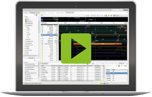
Screen Cast: Introducing the areas of the impulse viewer

The impulse Viewer

The impulse viewer UI consists of the four main areas shown in the picture of the user interface below, namely:

Plot Tree

The View Plot Tree contains a hierarchy of plots and folders. For each element in the tree, there is a corresponding visualization in the Plot Area.

Signal Area

The Signal Area's main use is to find signals in the record (wave, trace, log,..) file and convert them into a plot that can be shown in the Plot Area.

Plot Area

The Plot Area contains the main axis (possibly showing time, frequency, etc.), the waveform plots, and cursors. You can use a cursor or the scroll bar to select the visible domain range.

Cursor Details

The Cursor Details shows the list of all cursors, their actual domain value and the delta between the cursors.

Using the main menu of the viewer, you can configure the appearance of the viewer.

  • Show/Hide Signal Area
  • Show/Hide Cursor Details Area
  • Show/Hide Axis
  • Show/Hide Grid
  • Show/Hide Value Column
  • ....
  • Enable Fit Vertical

Fit Vertical tries to fit all plots into the vertical height of the viewer. If there is enough space, the elements are extended; if not, the elements are shown with minimal height. This can be very useful in the case of few plots (e.g., scope or charts).

Plot Tree

The Plot Tree contains a hierarchy of plots and folders. For each element in the tree, there is a corresponding visualization in the Plot Area.

Each plot configuration describe how a signal (or signals) shall be visualized. Such a configuration contains a name , a description, the color, the link to the signal, the diagram type and a lot more. To add a signal to a view you just drag and drop it (or multiple signals/scopes) into the Plot Tree. To modify a plot you need to select one (or multiple), open the context menu (right click) and select Edit (or double-click the plot -- or press Enter).

Reorganization of the elements is possible with drag and drop or copy and paste. Furthermore, you can add folders (context menu) and manage the signals the way that you like.

The Plot Tree consists of two columns: one showing the name and icon and the second displaying the current value of the signal at the active cursor.

Organize View

Organize your view in hierarchies of plots and folders.

Configure Plots

Describe how your signals shall be visualized.

Cursor value

The 2nd column show the signal value at the actual cursor position.

Signal Area

The Signal Area's main use is to find signals in the record (wave, trace, log,..) file and convert them into a plot that can be shown in the Plot Area. The Signal Area consists of two parts: the Scope Hierarchy and the Filtered Signal Table.
The Scope Hierarchy in the upper part of the area contains the record (wave, trace, log, ...) file and all its scopes, modules and subsystem organization.
Below you find check fields with the following use:

  • All children: The filter is applied not only to the direct children of the selected scope, but to all subsequent children as well.

The Filtered Signal Table in the lower part of the area contains all filtered (or unfiltered) signals of the selected scope:

  1. Filter signals using a text fragment
    • abc: Show signal if text contains 'abc'
  2. Filter signals using a regular expression - Indicate with any of: '[](){}|?*^$.'
    • ab[0-9]n? : Show signal if text contains 'abc0n', ....
  3. Filter signals using a numeric expression
    • 0.4 < 2.0: Show signal if value matches range - use float or integer numbers (e.g. 0.1; 12 ; 0x300)
    • < 0x400: ... if value less than argument
    • <=-4: ... if value less or equal than argument
    • > 2.7: ... if value greater than argument
    • >= 0.04: ... if value greater or equal than argument
    • == 1000: ... if value equals argument

Explore

Explore the contents of you record.

Search

Use filters to search for signals.

Create plots from signals

Create plots by dragging (or double-clicking) signals and scopes into the plot tree.

Plot Area

The Plot Area contains the main axis (possibly showing time, frequency, etc.), the waveform plots, and cursors. You can use a cursor or the scroll bar to select the visible domain range. The Plot Area allows you to:

  • Adjust the diagrams by changing the resolution (zoom) and time frame.
  • Step between changes in the signal.
  • Undertake quick measures.
  • Value inspection (double-click on the plot).
  • Search for signal patterns (CTRL-F).

Useful Shortcuts:

  • Zoom In (at active cursor)Ctrl +/Numpad +
  • Zoom Out (at active cursor) Ctrl - /Numpad -
  • Zoom Fit Ctrl */Numpad *
  • Zoom (at mouse) Shift Wheel
  • Zoom Range CtrlLeft Click / Move

Find

Find points of interrest by changing the resolution (zoom) and time frame. Enter Ctrl-F to open the find dialogue.

Inpsect and Measure

Undertake quick measures and double-click to open the Sample Inspector.

Annotate

Add Bookmarks and Annotations.

Cursor Details

Initially, this area is not visible but can be activated with the corresponding toolbar button.
The area contains:

  • A list of all cursors and their actual time (or any unit that is used for the x-axis).
  • A diagram that shows the delta between the cursors.

Overview

Get an overview of all cursors and their position.

Switch

Switch between cursors.

Delta

View the cursor delta values.
toem

technical software and tooling

Company

Contact Us

This email address is being protected from spambots. You need JavaScript enabled to view it.